Working as a ‘Spreadsheet Guy’ i use VLOOKUP every day and a lot of people comes to me with an issue saying “my vlookup is not working”, for one reason or another. VLOOKUP is a very common excel function (in fact the 3rd most used Excel Function). You have to admit, as much fun using VLOOKUP is, so frustrating are the errors associated with it. This is because of the limitations of VLOOKUP. Things will get easier in the future as Microsoft has announced XLOOKUP as a replacement for VLOOKUP. In this article, we are going to discuss 5 top reasons why your VLOOKUP is not working and how to fix them.
Types of Errors in VLOOKUP
Before we can solve the error it is important to know which kind of error you are getting and what can be the possible reasons for that error type. Excel VLOOKUP formula gives 3 main types of errors. Below are the 3 types of errors and what they possibly mean.
1. #VALUE!
This Error is the least common Error. The #VALUE! error occurs in two scenarios
- The lookup_value argument is more than 255 characters.
- The col_index_num argument contains text or is less than 0.
2. #REF!
The REF! stands for reference. Excel displays this error when a formula references a cell that no longer exists, usually caused by deleting the cells that formula is referring to. You can also notice this error when your table does not have that much range as mentioned in the col_index_num argument. You can solve this by fixing your col_index_num argument.
3. #N/A
This is the most common type of error in excel VLOOKUP function and probably the reason why your VLOOKUP is not working. N/A means Not Available and Excel gives this error when the lookup_value you are looking for is not found in the first column of the table_array of the VLOOKUP. Below we will discuss the top reasons why #N/A is showing up and how to fix it.
Top Reasons Why Your VLOOKUP is Not Working, and How to Fix Them
1. Numbers Formatted as Text
This is the most common cause of the #NA error When the lookup_value is a Number and the Table_array has the value formatted as Text, VLOOKUP can not search for the value. This scenario occurs when someone is trying to show the leading Zeros. To fix this issue all Numeric values must be formatted as Numbers. 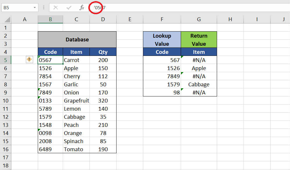
Solution: The cells containing Numeric values as text can be distinguished by a filled triangle on the Top-Left corner of the cell. Click on that cell and you can find a Caution Symbol, click on it and choose Convert to Number. This will also work on a cell range.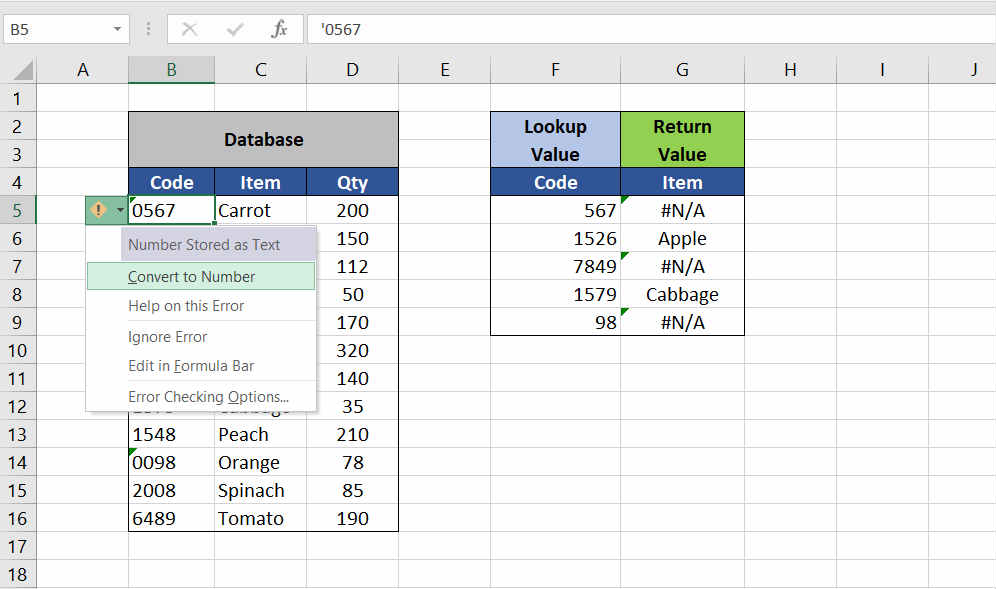
Also, you can Multiply your range by 1 to convert it to Numbers. Just write 1 in any blank cell and copy it, then select your range and press CTRL+ALT+V and select Multiply operation.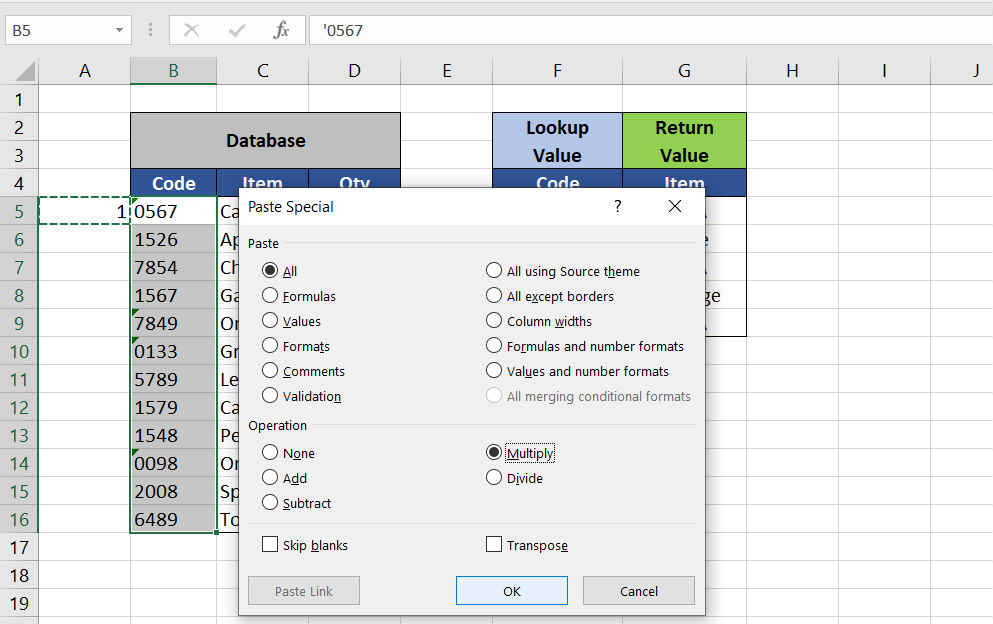
2. Table Array is not Reference Locked
When you are using VLOOKUP for a range and you drag down the formula to copy it down. But now only half of the formulae are working and you wonder why? As you can see in the example below you can see as you copy your formula down with each cell the Table_array is also shifting down
Solution: After selecting the table_array in your formula press F4 to Reference lock your table_array before you copy your formula down. It is a good practice.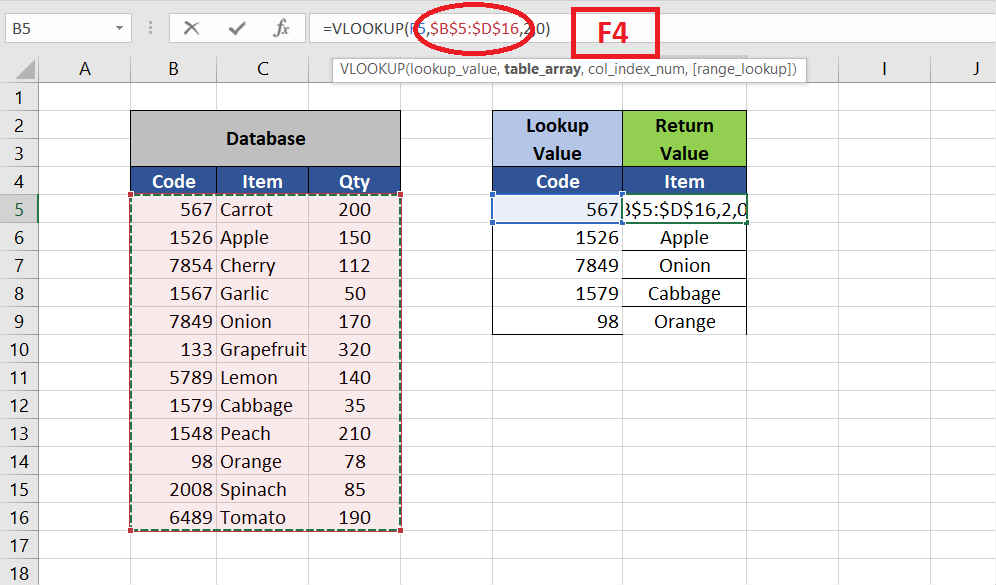
3. Leading or Trailing Spaces at the End of the Value
Look at the example below, the formula and data look absolutely correct yet it is showing #NA error and the VLOOKUP is not working 100 percent. The Problem here is invisible to the naked eye. To see this go to the lookup value and put your cursor at the end in the formula bar, you can see some leading and trailing spaces in your lookup value. The VLOOKUP formula doesn’t work with extra spaces.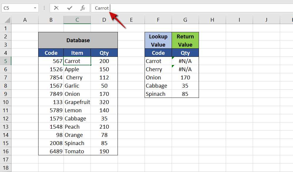
Solution: To clean your data by removing the extra useless spaces you can use the TRIM command. The trim command removes all the leading and trailing spaces of your value. You can use the TRIM command in separate dummy sheet and once your data set is trimmed you can Copy-Paste it as Values to its destination. OR you can change your formula as
=VLOOKUP(TRIM(Lookup_Value), Table_Array, Col_Index_Num,[Range_Lookup])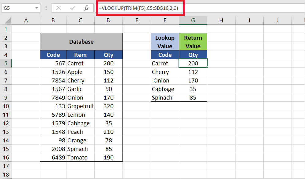
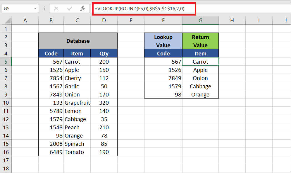
4. The Numbers are Fraction
It is wise to use VLOOKUP only with Integers. The VLOOKUP will show #NA error when one of the lookup_value or Table_array value is a fraction. The value might look like an Integer because of the Number Formatting but you can check the actual Fraction in the formula bar. See the example below.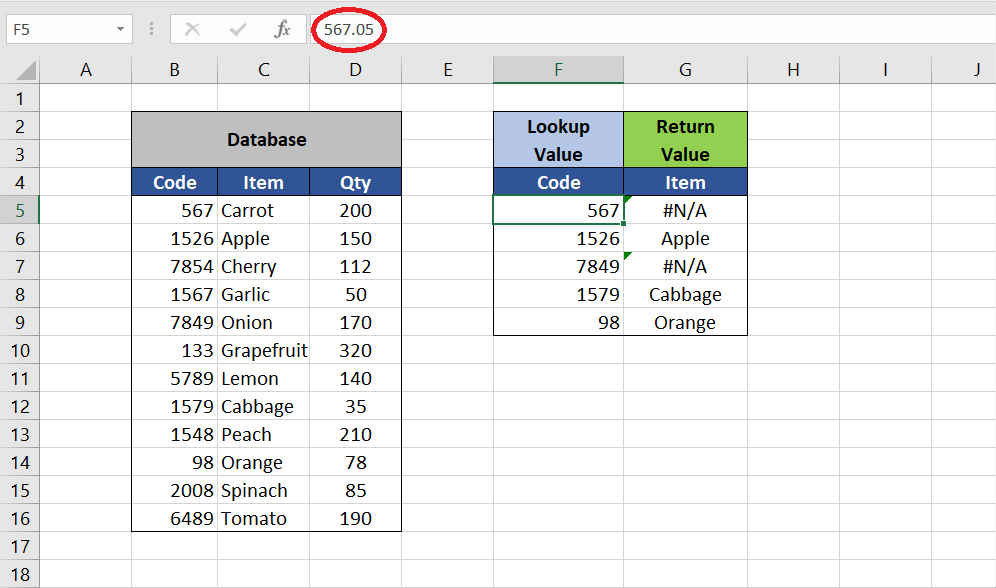
Solution: To Get rid of the Fractions from your Data set, you can use the ROUND function. ROUND function coverts the fractions to the Integer value. Once you Round up your range you can copy-paste it back as values. OR you can write up your formula as
=VLOOKUP(ROUND(Lookup_Value,0), Table_Array, Col_Index_Num,[Range_Lookup])
5. Change of Calculation Option:
If all your Formulae are correct and none of them are working even after spending hours debugging the formula you might want to take a look at the Calculation Options. Sometimes the calculation options can get set to ‘Manual’ and stop all your formulae to work automatically. To reset it to Automatic go to Formula tab click on the Calculation option and set it to Automatic.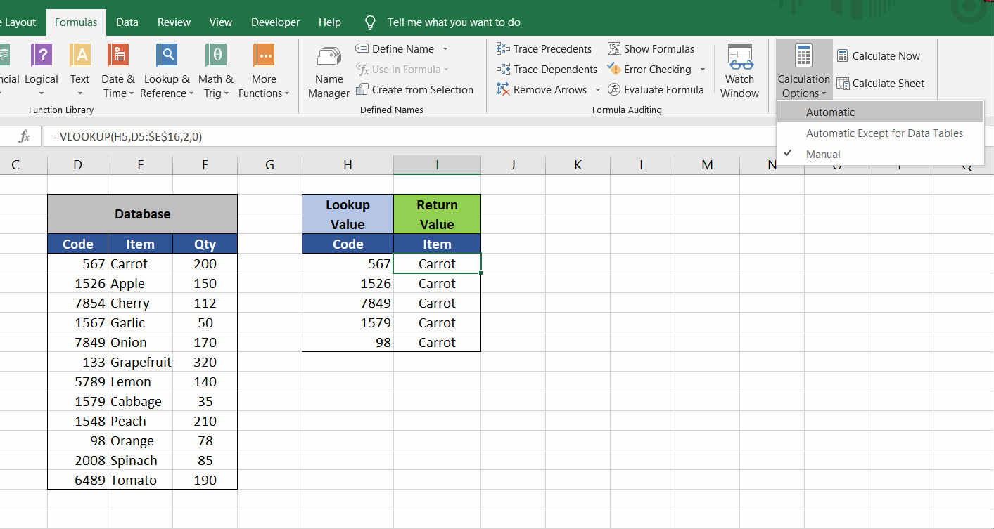
Formula Tab → Calculation Options → Automatic
So these were the top reasons why your VLOOKUP formula is not working. If you found it useful or if u have any other excel doubts please mention in the comments below. Also, suggest in comments if you have some more ideas.
Thank you!